Four Effects of Financial Venturi on Significant Stock Market Profits

What is causing this stock market crash, which is not supported by unusually strong fiscal flows and faces a normal seasonal pattern?

The table below shows the most recent US sector balances. Month. This information is compiled from the United States National Accounts.

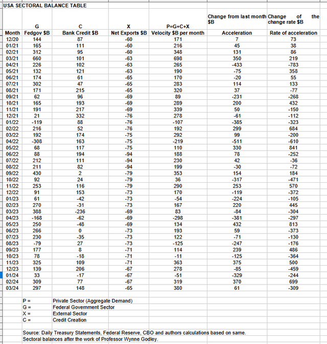
In March 2024, the private sector recorded a surplus of $380 billion. This is a very positive outcome for asset markets, as private sector financial balances have increased and aggregate demand for goods, services and investment assets has increased.

From this table, we can see that the $380 billion in private funds surplus was due to a $297 billion infusion by the federal government (which included about (Includes $8 billion in new injection channels from the Fed). Banking sector) minus $65 billion that flowed from the domestic private sector to the Fed’s foreign bank accounts (External sector X) in exchange for imported goods and services. Bank credit creation added him $148 billion, more than double what he had last month.

The numbers for the past six months or so are no more unusual than they were during the 2020 coronavirus emergency spending and stock market recovery shown at the top of the table. Fiscal flows alone cannot explain the sudden and sustained collapse of the US stock market.

The table below shows the amounts withdrawn by the federal government from Federal Reserve bank accounts. When the government spends money, more money is given to the private sector, leading to a rise in the stock market.

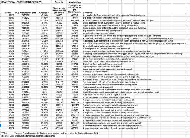
The table shows that total spending is down nearly $5 trillion compared to the previous month, to around $2.5 trillion. This month, federal taxes, fees, charges, and bond sales left $297 billion of spending in the private sector, creating a federal deficit equal to the private sector surplus. Subtracting the current account deficit from this result leaves the domestic private sector balance at $228 billion. In terms of purchasing power, this increases again with the addition of $148 billion in bank credit creation.

While this is a strong result, it is not strong enough to explain the stock market’s strength over the past six months.

The chart below shows how changes in the US private and domestic sector balance tend to lead the SPX.

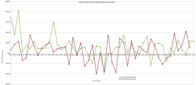
Last month, Domestic Private Sector Balance’s Lead over (SPX) predicted that (SPX) would end March higher than it started, and that’s exactly what happened.

This month’s graph predicts a similar outcome for April, given that domestic private sector fiscal flows remain strong. So far, this has been the case and may continue to be the case.

The chart below shows how the US sector balance sheet information changes over time, taking into account the lagged effects of these changes. It’s like a tool that helps you see what’s happening in the market from a distance.

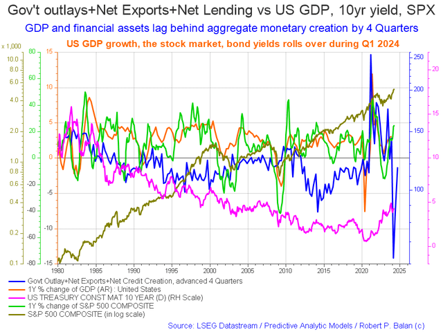
The blue line represents the money spent by the government and the credit generated by banks minus current account balances. Predict economic changes up to four quarters in advance.

The change from last month is that SPX is up and so are GDP and bond yields. The first blue line continues to rise.

The chart below shows the five-year average of seasonal stock market patterns for SPX (SPX), Nasdaq (NDX), Dow (DIA), Russell 2000 (RTY), and the biotech market index. The black oval shows where we are currently.

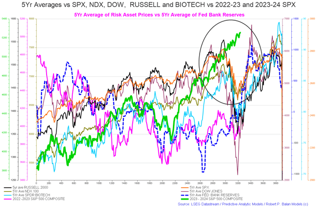
This graph clearly shows how the green line ignores the expected seasonal pattern set by the orange line. The orange line is his five-year average for SPX. Originally, SPX should have fallen by the end of his first quarter of 2024, giving him an opportunity to buy on the spurt. There should have been at least two seasonal buy-in opportunities this year, but they didn’t materialize, and some are wondering why.

Four factors come to mind.

1. Treasury interest income due to interest rate increases.

2. Global fiscal spending by world governments.

3. The upcoming peak of the real estate cycle.

4. Interest paid by the Federal Reserve to banks on reserve balances increases with interest rates.

These factors are discussed in more detail below.

1. Treasury interest income:

One of the big things that has changed over the past 18 months or so is the Fed and its interest rate policy position.

What’s different from previous years is that interest rates are now higher, but that’s simply because wealthy recipients are pushing up Treasury revenues, allowing them to buy paper in a narrowly focused way, beyond the scale of their normal asset purchase patterns. They may just be buying assets.

The graph below shows the very long-term and broad-based growth relationship between federal interest spending and the stock market.

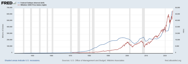
Federal government interest spending has led the stock market for several quarters, and the curve appears to be steepening over time, with that effect accelerating as the Treasury inventory grows. The curve is now almost vertical.

2. Convergence of G5 fiscal flows and increasing time difference effects.

G5 flows are the sum of the spending of the world’s five largest economies. C5 is the balance sheet of the world’s five largest central banks.

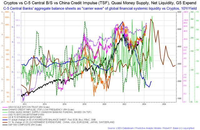
Together, G5 and C5 fiscal flows affect what is known in fluid mechanics as the carrier wave that underlies all other fiscal flows and market effects.

The chart above shows that the brown carrier wave is rising sharply towards 2024, which will also tend to lift the asset market.

The brown line in the chart above shows this carrier. The following graph shows this in a more detailed form, but it is not as detailed as the graph above.

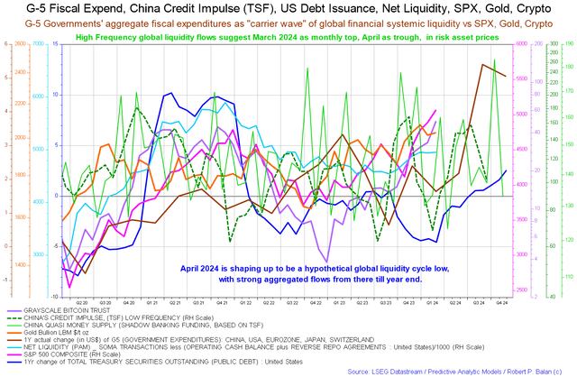
A short-term view of the same information shows how the brown line will decline in the first quarter of this year and rise from the second quarter onwards.

These charts are not very detailed, and the macro rally from the G5 flow could arrive sooner than expected, explaining the market’s unusual dynamism. It also points to the fact that the situation is likely to get better, not worse, as the year progresses.

3. The economic rent impact of the last mania-driven winner will have a negative impact on the real estate cycle.

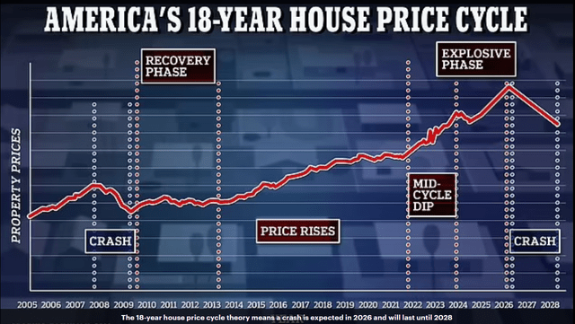
The graph above shows the progression of the real estate cycle and how it is now entering its last, most explosive and speculative phase. Rising real estate prices have created a concentrated wealth effect for property owners, reaching the peak of price increases since the recovery began in 2009. Fifteen years of land price growth peaked, monetized, and then entered the asset market.

Land prices rise so much that they reach a peak, creating a wealth effect based on the value of ordinary people’s homes. Some of them will be able to obtain home equity loans and use the wealth they have acquired out of thin air to convert into paper assets, further contributing to the stock market crash in a concentrated manner. There, we see how rising land prices foster credit creation, which aggregates demand not just in the corners of the city, but also among ordinary people, and how this capital flows intensively into the stock market.

The housing market is closely linked to the overall economy and is expected to reach its highest point in 2026, so it’s important to check it regularly.

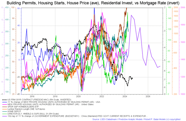
This chart shows aspects of the housing market. In this example, the price of lumber (the orange line, which tends to rise during booms) appears to have bottomed out and is approaching a local low, but has not yet risen. Currently, only Home Depot, a home construction ETF, is down month-over-month. Despite this, housing starts and permits increased.Freddie Mac’s 30-year contract rate declines [which is normally good for housing and may explain why permits and approval increased at the same time as more people took on a slightly cheaper loan and chose to build or buy] What’s important to note, however, is that the purple government spending line rises through most of the rest of 2024, then falls, and then rises again in 2025. This line is the same financial career wave that determines the overall trend of all other waves that follow. Shown in point 2 above.

4. Interest on Federal Reserve Reserve Balances

Another important factor is the interest on reserve income that flows directly to banks as a result of high interest rates, and is related to the first factor above.This is shown in the graph below

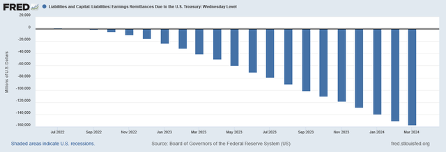
Banks tend to invest their surplus income in high-yielding paper assets such as stocks and bonds at a rate of about $10 billion per month.

4-way financial venturi effect.

The four factors above support the thought experiment that the current and continuing stock market crash in the face of average financial flows alone is caused by the financial Venturi effect.

Treasury interest income, IORB, monetized wealth from real estate cycles are sources of income when the majority of recipients are already wealthy. Recipients seek to invest this money in paper assets in search of yield and high levels of discretionary spending, resulting in a stock market rally that is out of proportion to the actual strength of current fiscal flows. Masu.

The background effect of an overall increase in the lagged impact of G5 fiscal flows supports and strengthens this Venturi effect.